Statistical testing using R

Data

Load the data set into R environment. This data set is collect by Walmart for researching variables that might influence the CPI score (Consumer price index).
[DOWNLOAD HERE]

data = read.csv('../data/walmart.csv')
head(data)
A data.frame: 6 × 9
Store year month day Temperature Fuel_Price CPI Unemployment IsHoliday
<int> <int> <int> <int> <dbl> <dbl> <dbl> <dbl> <lgl>
1 1 2010 2 5 42.31 2.572 211.0964 8.106 FALSE
2 1 2010 2 12 38.51 2.548 211.2422 8.106 TRUE
3 1 2010 2 19 39.93 2.514 211.2891 8.106 FALSE
4 1 2010 2 26 46.63 2.561 211.3196 8.106 FALSE
5 1 2010 3 5 46.50 2.625 211.3501 8.106 FALSE
6 1 2010 3 12 57.79 2.667 211.3806 8.106 FALSE

Simple plots

Making some simple plots is a smart way of knowing our data set in the first stage. Try to make all following plots. What conclusion can you make by observing?

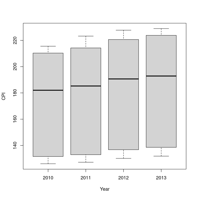
  1. A side-by-side boxplot
plot(x = factor(data$year), y = data$CPI, xlab = "Year", ylab = "CPI")

  1. A scatter plot. x: Unemployment, y: CPI
plot(x = data$Unemployment, y = data$CPI, pch = 20, xlab = "Unemployment", ylab = "CPI")

Descriptive statistics

Calculate sample size, Mean, SD, variance, IQR of CPI each year and present it in a table. This should be a data frame or a matrix with six columns.

tab = data.frame(year=unique(data$year), Count=NA, Mean=NA, SD=NA, Variance=NA, IQR=NA)
for(y in unique(data$year)){
    cpiYear = data$CPI[data$year == y]

    tab$Count[tab$year == y] = sum(! is.na(cpiYear))
    tab$Mean[tab$year == y] = mean(cpiYear, na.rm=T)
    tab$SD[tab$year == y] = sd(cpiYear, na.rm=T)
    tab$Variance[tab$year == y] = var(cpiYear, na.rm=T)
    tab$IQR[tab$year == y] = IQR(cpiYear, na.rm=T)
}

print(tab)
  year Count     Mean       SD Variance      IQR
1 2010  2160 168.1018 38.22239 1460.951 78.74260
2 2011  2340 171.5457 38.98675 1519.966 81.28978
3 2012  2340 175.7166 40.79858 1664.524 83.89305
4 2013   765 177.6088 41.51821 1723.762 85.28620

t-test

  1. Test if the CPI score in 2010 and 2012 are the same.
    • Assume that the population variances are not the same. Which t-test should you choose?
    • What’s your hypothesis? (H0 vs H1)
    • Driven the test in R. What is your conclusion?
cpi2010 = data$CPI[data$year == 2010]
cpi2012 = data$CPI[data$year == 2012]
t.test(cpi2010, cpi2012, var.equal=F)

    Welch Two Sample t-test

data:  cpi2010 and cpi2012
t = -6.4642, df = 4497, p-value = 1.127e-10
alternative hypothesis: true difference in means is not equal to 0
95 percent confidence interval:
 -9.924313 -5.305366
sample estimates:
mean of x mean of y 
 168.1018  175.7166 
  1. Test if the fuel price in 2010 and 2012 are the same. Then, assume that the population variance is the same.
    • Which t-test should you choose?
    • What’s your hypothesis?
    • Driven it in R, and what’s your conclusion?
fuel2010 = data$Fuel_Price[data$year == 2010]
fuel2012 = data$Fuel_Price[data$year == 2012]
t.test(fuel2010, fuel2012, var.equal=T)

    Two Sample t-test

data:  fuel2010 and fuel2012
t = -119.71, df = 4498, p-value < 2.2e-16
alternative hypothesis: true difference in means is not equal to 0
95 percent confidence interval:
 -0.8622102 -0.8344239
sample estimates:
mean of x mean of y 
 2.823767  3.672084 

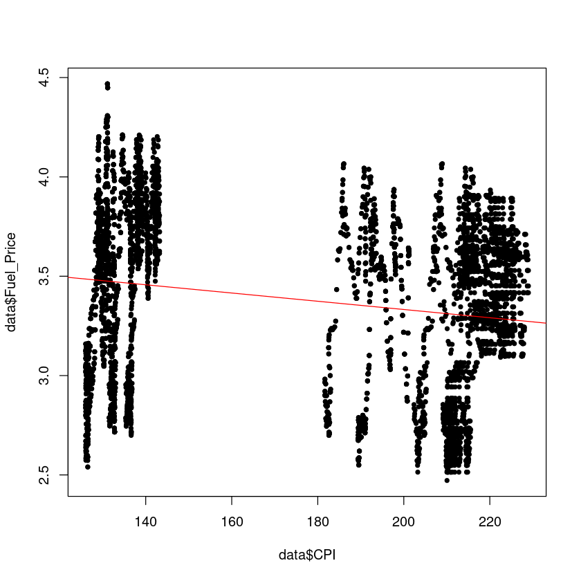
Correlation coefficient

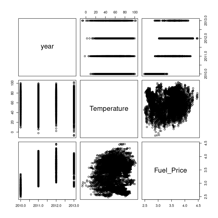
Calculate the pairwise correlation between year, temperature, and fuel price. Present it in both the plot (scatter plot) and correlation matrix.

cor(data[, c(2, 5, 6)])
A matrix: 3 × 3 of type dbl
year Temperature Fuel_Price
year 1.00000000 -0.03837331 0.6577771
Temperature -0.03837331 1.00000000 0.1013542
Fuel_Price 0.65777712 0.10135422 1.0000000
plot(data[, c(2, 5, 6)])

Advanced

Try this section after you finish all previous sections

Fancy plots

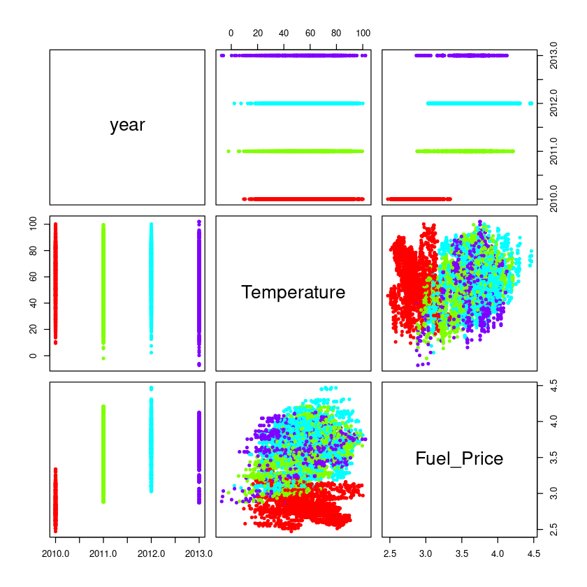
  • Paint scatter plot by years.
pairs(data[, c(2, 5, 6)], pch = 20, col = rainbow(4)[factor(data$year)])

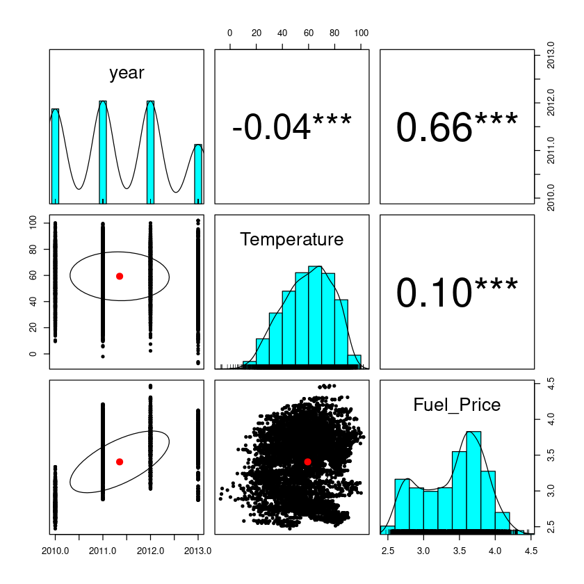
  • Add density plot, correlation coefficient score, and confidence interval. (HINT: ??pairs.panels)
# install.packages('psych')
library(psych)
pairs.panels(
    data[, c(2, 5, 6)],
    smooth = F,
    density = T,
    method = "pearson",
    pch = 20,
    lm = FALSE,
    stars = TRUE,
    ci = TRUE
)

The simple linear regression model

Fit a simple linear regression model with - Independent variable: CPI (x) - Dependent variable: Fuel price (y)

Answer the following questions. - What is the p-value in the returned table stand for? - What is the formula of this model?

fit = lm(Fuel_Price ~ CPI, data)
summary(fit)

Call:
lm(formula = Fuel_Price ~ CPI, data = data)

Residuals:
    Min      1Q  Median      3Q     Max 
-0.9449 -0.4276  0.1134  0.3431  0.9926 

Coefficients:
              Estimate Std. Error t value Pr(>|t|)    
(Intercept)  3.7473154  0.0221518  169.17   <2e-16 ***
CPI         -0.0020740  0.0001252  -16.57   <2e-16 ***
---
Signif. codes:  0 ‘***’ 0.001 ‘**’ 0.01 ‘*’ 0.05 ‘.’ 0.1 ‘ ’ 1

Residual standard error: 0.4337 on 7603 degrees of freedom
  (585 observations deleted due to missingness)
Multiple R-squared:  0.03486,   Adjusted R-squared:  0.03473 
F-statistic: 274.6 on 1 and 7603 DF,  p-value: < 2.2e-16

Draw the scatter plot and the fitted regression line.

plot(data$Fuel_Price~data$CPI, pch=20)
abline(a=3.7473154, b=-0.0020740, col='red')

Draw the residuals plot. Does the variance of CPI well explain by the fuel price?

plot(x = fit$fitted.values,y = fit$residual, pch = 20, xlab = "Fitted value", ylab = "Residual")
abline(h = 0, col='red')

Discrete data

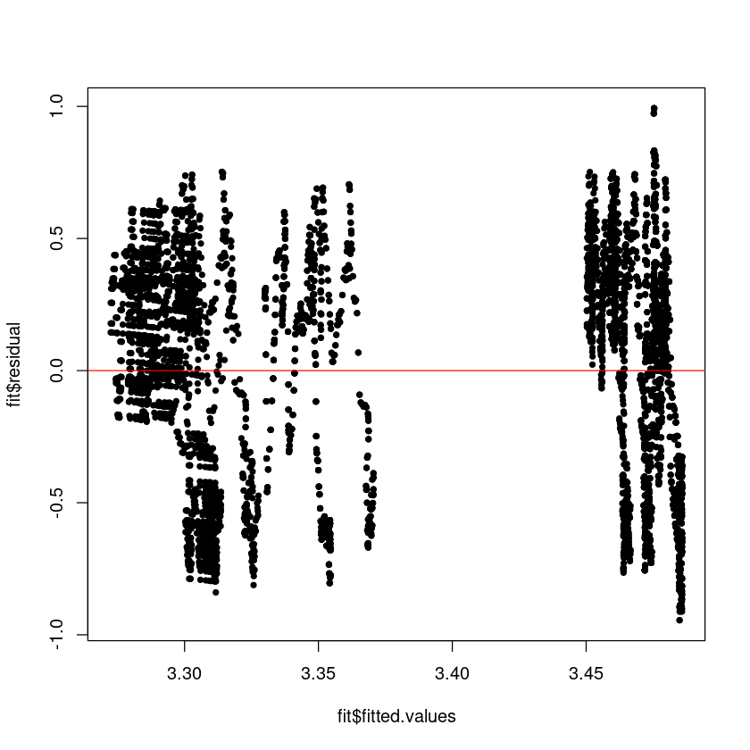
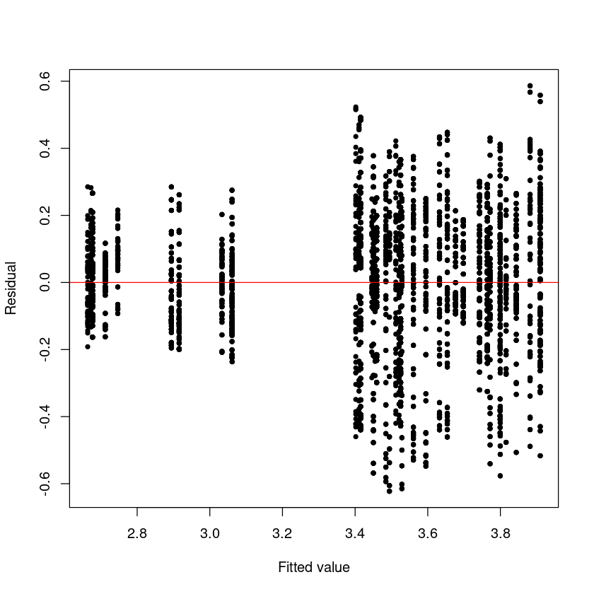
This section will try to fit a linear model with independent variables having a discrete data type.

Fit store, year, temperature, fuel price, and unemployment rate into the model. Note that store and year should be considered category data in this case.

This will return a long table. When we consider category information as a dependent variable, using a dummy variable is how we calculate.

  • What are the reference points for stores and years?
fit = lm(Fuel_Price ~ factor(Store) + factor(year), data)
summary(fit)

Call:
lm(formula = Fuel_Price ~ factor(Store) + factor(year), data = data)

Residuals:
     Min       1Q   Median       3Q      Max 
-0.62247 -0.11065  0.00925  0.13084  0.58626 

Coefficients:
                   Estimate Std. Error t value Pr(>|t|)    
(Intercept)       2.677e+00  1.526e-02 175.405  < 2e-16 ***
factor(Store)2    1.142e-15  2.094e-02   0.000 1.000000    
factor(Store)3    3.277e-15  2.094e-02   0.000 1.000000    
factor(Store)4   -4.357e-03  2.094e-02  -0.208 0.835203    
factor(Store)5    4.094e-15  2.094e-02   0.000 1.000000    
factor(Store)6    1.491e-15  2.094e-02   0.000 1.000000    
factor(Store)7    3.516e-02  2.094e-02   1.679 0.093239 .  
factor(Store)8    4.210e-15  2.094e-02   0.000 1.000000    
factor(Store)9    4.456e-15  2.094e-02   0.000 1.000000    
factor(Store)10   3.564e-01  2.094e-02  17.017  < 2e-16 ***
factor(Store)11   2.702e-15  2.094e-02   0.000 1.000000    
factor(Store)12   3.844e-01  2.094e-02  18.355  < 2e-16 ***
factor(Store)13   6.952e-02  2.094e-02   3.319 0.000906 ***
factor(Store)14   2.172e-01  2.094e-02  10.369  < 2e-16 ***
factor(Store)15   3.841e-01  2.094e-02  18.340  < 2e-16 ***
factor(Store)16   3.516e-02  2.094e-02   1.679 0.093239 .  
factor(Store)17   6.952e-02  2.094e-02   3.319 0.000906 ***
factor(Store)18   2.386e-01  2.094e-02  11.394  < 2e-16 ***
factor(Store)19   3.841e-01  2.094e-02  18.340  < 2e-16 ***
factor(Store)20   2.172e-01  2.094e-02  10.369  < 2e-16 ***
factor(Store)21   2.845e-15  2.094e-02   0.000 1.000000    
factor(Store)22   2.386e-01  2.094e-02  11.394  < 2e-16 ***
factor(Store)23   2.386e-01  2.094e-02  11.394  < 2e-16 ***
factor(Store)24   3.841e-01  2.094e-02  18.340  < 2e-16 ***
factor(Store)25   2.172e-01  2.094e-02  10.369  < 2e-16 ***
factor(Store)26   2.386e-01  2.094e-02  11.394  < 2e-16 ***
factor(Store)27   3.841e-01  2.094e-02  18.340  < 2e-16 ***
factor(Store)28   3.844e-01  2.094e-02  18.355  < 2e-16 ***
factor(Store)29   2.386e-01  2.094e-02  11.394  < 2e-16 ***
factor(Store)30   2.650e-16  2.094e-02   0.000 1.000000    
factor(Store)31   1.386e-15  2.094e-02   0.000 1.000000    
factor(Store)32   3.516e-02  2.094e-02   1.679 0.093239 .  
factor(Store)33   3.564e-01  2.094e-02  17.017  < 2e-16 ***
factor(Store)34  -4.357e-03  2.094e-02  -0.208 0.835203    
factor(Store)35   2.172e-01  2.094e-02  10.369  < 2e-16 ***
factor(Store)36  -1.330e-02  2.094e-02  -0.635 0.525527    
factor(Store)37   8.414e-16  2.094e-02   0.000 1.000000    
factor(Store)38   3.844e-01  2.094e-02  18.355  < 2e-16 ***
factor(Store)39   1.139e-15  2.094e-02   0.000 1.000000    
factor(Store)40   2.386e-01  2.094e-02  11.394  < 2e-16 ***
factor(Store)41   3.516e-02  2.094e-02   1.679 0.093239 .  
factor(Store)42   3.564e-01  2.094e-02  17.017  < 2e-16 ***
factor(Store)43   1.055e-15  2.094e-02   0.000 1.000000    
factor(Store)44   6.952e-02  2.094e-02   3.319 0.000906 ***
factor(Store)45   2.172e-01  2.094e-02  10.369  < 2e-16 ***
factor(year)2011  7.381e-01  5.961e-03 123.822  < 2e-16 ***
factor(year)2012  8.483e-01  5.961e-03 142.302  < 2e-16 ***
factor(year)2013  7.823e-01  6.932e-03 112.858  < 2e-16 ***
---
Signif. codes:  0 ‘***’ 0.001 ‘**’ 0.01 ‘*’ 0.05 ‘.’ 0.1 ‘ ’ 1

Residual standard error: 0.1998 on 8142 degrees of freedom
Multiple R-squared:  0.7867,    Adjusted R-squared:  0.7855 
F-statistic: 638.9 on 47 and 8142 DF,  p-value: < 2.2e-16

Draw the residual plot again. Does CPI be explained better in this model?

plot(x = fit$fitted.values,y = fit$residual, pch = 20, xlab = "Fitted value", ylab = "Residual")
abline(h = 0, col='red')

ANOVA

Fit a two-way ANOVA model: CPI = Store + year + e. - Do your degrees of freedom make sense? (If it is 1, you may forget to convert your data type as factor) - What conclusion can you make from this result?

fit = aov(Fuel_Price ~ factor(Store) + factor(year), data)
summary(fit)
                Df Sum Sq Mean Sq F value Pr(>F)    
factor(Store)   44  189.8     4.3     108 <2e-16 ***
factor(year)     3 1008.8   336.3    8424 <2e-16 ***
Residuals     8142  325.0     0.0                   
---
Signif. codes:  0 ‘***’ 0.001 ‘**’ 0.01 ‘*’ 0.05 ‘.’ 0.1 ‘ ’ 1