#> tar -xvf human.tar.gzQuality Control
You are highly recommended to work on the server today. The first part of this practice will need to run PLINK and vcftools.
Dataset
- Copy the dataset to your working directory from
/proj/g2020004/nobackup/oumark/gwas_lab2/human.tar.gzon UPPMAX. - Unzip the
human.tar.gz - After unzipping the folder, you will have
human.bed,human.bim, andhuman.famthree files. We call this kind of format as PLINK binary files.
A quick view
Before we start all QC jobs, let’s have a quick view of our data. First, find answers to the following questions from PLINK’s website.
FAM file
Have a look at human.fam in terminal
- Which column is the family ID (FID)? What is the prefix?
- Which column is the Within-family ID (IID)? What is the prefix?
- Does this dataset provide parental information? What does 0 stands for?
- How many samples are included in this dataset?
BIM file
Have a look at human.bim in terminal
- What does each column mean?
- How does the missing value present in the columns for reference and alternative alleles?
- How many markers are included in this dataset?
PLINK
- Homepage: https://www.cog-genomics.org/plink/1.9/
Data input
Several data formats are available for PLINK. The dataset we provide for today’s practice is the PLINK 1 binary format. Have a look at the help manual on how to load the dataset. LINK
Here are some tricks to make your work easier: - The prefix of the three files should be the same. - Make sure all three files are placed in the same directory.
Data output
One powerful function of PLINK is converting the dataset format used in other software. Have a look at the help manual for the output format option. LINK
- Input the PLINK binary file and generate a block-gzipped VCF file. (this will be used in the next section)
- What’s the function of
--outoption? - Have a look at the message in the terminal. How many variants are loaded from the BIM file? How many males and females sample were loaded?
- Do you find your output file human.vcf.gz?
- What’s the function of
#> plink --bfile human --recode vcf bgz --out humanTry following QC options
Try to filter the dataset by the following steps and write down the number of markers and samples passed in each step. (Note: output name needs to be changed in each run)
- Minor allele frequency (0.01)
#> plink --bfile human --maf 0.01 --make-bed --out human_maf- Individual genotyping rate (0.05 missingness)
#> plink --bfile human_maf --mind 0.05 --make-bed --out human_maf_mind- SNP genotype rate (0.05 missingness)
#> plink --bfile human_maf_mind --geno 0.05 --make-bed --out human_maf_mind_geno- Hardy-Weinberg P (0.001)
#> plink --bfile human_maf_mind_geno --hwe 0.001 --make-bed --out human_maf_mind_geno_hweAfter doing all steps, - How many markers remain in the dataset? - How many samples remain in the dataset?
All in a run
Perform all steps from the raw data in one run by PLINK. - Does the number of remaining markers and samples differ from the step-by-step result? Why?
#> plink --bfile human --maf 0.01 --mind 0.05 --geno 0.05 --hwe 0.001 --make-bed --out human_allVCFtools
- Homepage: https://vcftools.github.io/index.html
- Use the
human.vcf.gzyou generated in the previous section.
Data input
- What are the avalible input formats for this software? Which option should we use for our dataset?
Data output
- What are the output options?
- What is the command for output VCF format? a 012 matrix for genotype? and PLINK format?
Try QC options
Try to filter your dataset by the following instructions and write down the number of remaining markers and samples after filtering.
- Minor allele frequency (0.1)
#> vcftools --gzvcf human.vcf.gz --maf 0.01 --recode --stdout | gzip -c > human_maf.vcf.gz- Include only bi-allelic sites
#> vcftools --gzvcf human_maf.vcf.gz --min-alleles 2 --max-alleles 2 --recode --stdout | gzip -c > human_maf_bil.vcf.gz- SNP genotype rate (0.05 missingness)
#> vcftools --gzvcf human_maf_bil.vcf.gz --max-missing 0.05 --recode --stdout | gzip -c > human_maf_bil_geno.vcf.gz- Hardy-Weinberg P (0.001)
#> vcftools --gzvcf human_maf_bil_geno.vcf.gz --hwe 0.001 --recode --stdout | gzip -c > human_maf_bil_geno_hwe.vcf.gzAll in a run
Perform all QC steps in one run and compare the result with the step-wise method.
#> vcftools --gzvcf human.vcf.gz --maf 0.01 --min-alleles 2 --max-alleles 2 --max-missing 0.05 --hwe 0.001 --recode --stdout | gzip -c > human_all.vcf.gzVisualization in R [ADVANCED]
Load data to R
read_plink()function in thegeniopackage is a powerful tool to read PLINK binary files.- Use PLINK binary files passed all QC in one run in the previous section.
library(genio)
data = read_plink('../data/human/human_all')
Reading: ../data/human/human_all.bim
Reading: ../data/human/human_all.fam
Reading: ../data/human/human_all.bed
Genotype frequency
Calculate genotype (0: A1A1, 1: A1A2, 2: A2A2) frequencies of each loci - Generate an empty data frame with three columns (A1A1, A1A2, A2A2). - Number of rows = number of markers
freq = data.frame(A1A1 = rep(NA, nrow(data$bim)), A1A2=NA, A2A2=NA)Use for loop to count the number of genotypes in each marker and divide by the number of samples.
#> nSmp = nrow(data$fam)
#>
#> for(i in 1:nrow(data$bim)){
#>     tmp = data$X[i, ]

#>     freq$A1A1[i] = sum(tmp == 0, na.rm = T) / nSmp
#>     freq$A1A2[i] = sum(tmp == 1, na.rm = T) / nSmp
#>     freq$A2A2[i] = sum(tmp == 2, na.rm = T) / nSmp
#> }
Bind frequency table with the marker information (HINT: cbind function can bind two data-frame)
freq = cbind(data$bim, freq)
head(freq)| chr | id | posg | pos | alt | ref | A1A1 | A1A2 | A2A2 | |
|---|---|---|---|---|---|---|---|---|---|
| <chr> | <chr> | <dbl> | <int> | <chr> | <chr> | <dbl> | <dbl> | <dbl> | |
| 1 | 1 | rs3094315 | 0.792429 | 792429 | G | A | 0.7528090 | 0.23595506 | 0.0000000 |
| 2 | 1 | rs4040617 | 0.819185 | 819185 | G | A | 0.7752809 | 0.22471910 | 0.0000000 |
| 3 | 1 | rs4075116 | 1.043550 | 1043552 | C | T | 0.8876404 | 0.11235955 | 0.0000000 |
| 4 | 1 | rs9442385 | 1.137260 | 1137258 | T | G | 0.3932584 | 0.40449438 | 0.1910112 |
| 5 | 1 | rs11260562 | 1.205230 | 1205233 | A | G | 0.9213483 | 0.05617978 | 0.0000000 |
| 6 | 1 | rs6685064 | 1.251210 | 1251215 | C | T | 0.4157303 | 0.34831461 | 0.2359551 |
Make a plot using the following scripts
library(tidyverse)

# prepare plotting data
plotDat = freq %>%
    as_tibble() %>%
    mutate(chr = as.numeric(.$chr), pos = as.numeric(.$pos))

plotDat = plotDat %>%
    group_by(chr) %>%
    summarise(chr_len = max(pos)) %>%
    mutate(tol = cumsum(chr_len) - chr_len) %>%
    left_join(plotDat, .) %>%
    arrange(chr, pos) %>%
    mutate(pos.cum = pos + tol) %>%
    select(chr, id, ref, alt, A1A1, A1A2, A2A2, pos.cum) %>%
    ungroup()
plotDat = pivot_longer(plotDat, cols = 5:7, names_to = "genotype", values_to = "frequency")

axisdf = plotDat %>%
    group_by(chr) %>%
    summarise(center = (max(pos.cum) + min(pos.cum))/2)

# Plot
p = ggplot(data = plotDat, aes(x = pos.cum, y = frequency, fill = genotype)) +
    geom_area(position = 'fill') +
    labs(x = "Chromosome", y = 'Frequency') +
    scale_x_continuous(label = axisdf$chr, breaks = axisdf$center) +
    theme_bw() +
    theme(panel.grid.major.x = element_blank(), panel.grid.minor.x = element_blank())
#ggsave('images/GTfrequency.jpeg', p)
Joining with `by = join_by(chr)`
Saving 6.67 x 6.67 in image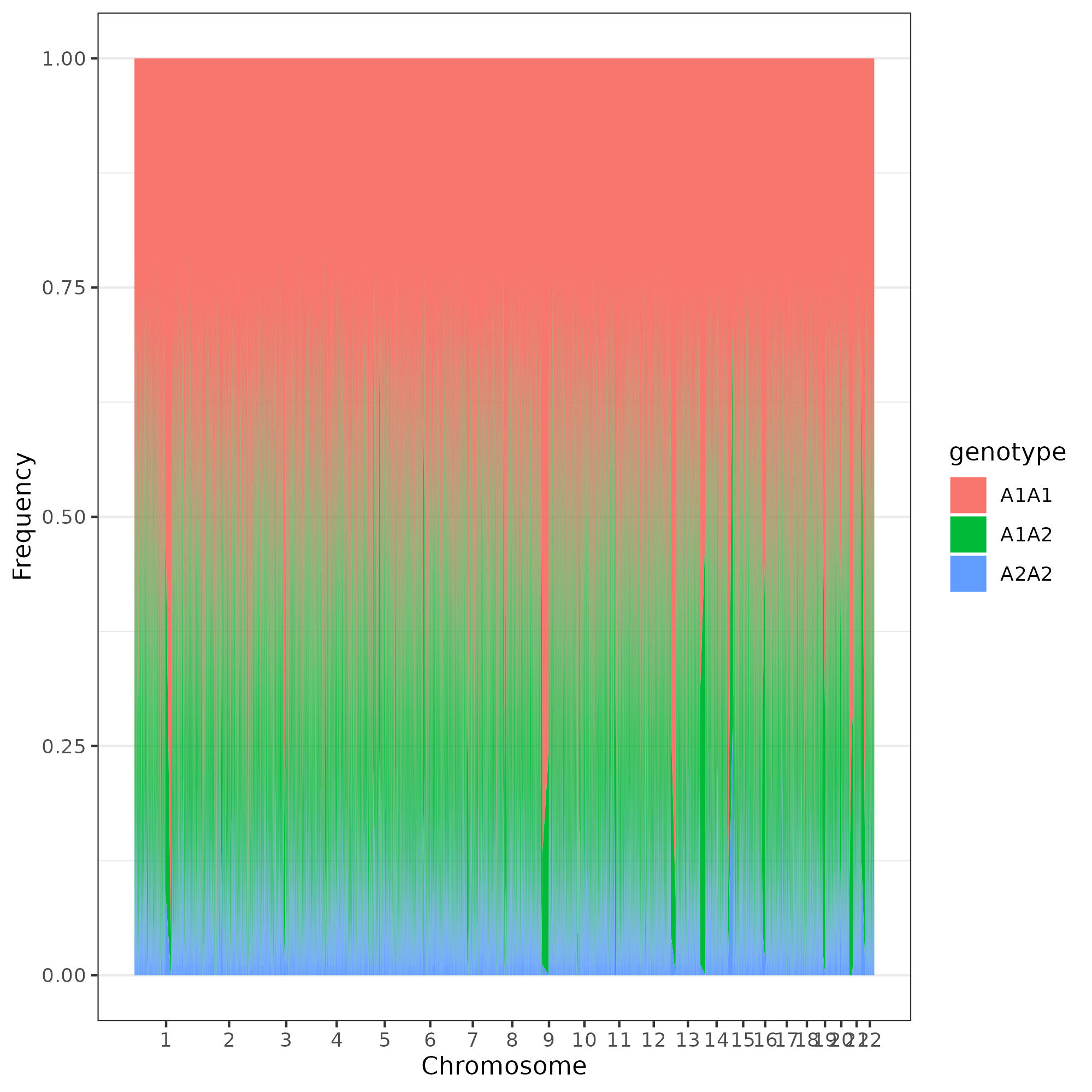
Questions: - Why visualizing dataset important? - Try calculate raw allele counts for each site by VCFtools. - What is the problem with low MAF? Is it a good idea to have a stricter rule for MAF (a higher MAF threshold)? Why?