exampleData = data.frame(
    case = c(20, 20, 60),
    control = c(50, 30, 20)
)

result = chisq.test(exampleData)
print(result)
    Pearson's Chi-squared test

data:  exampleData
X-squared = 34.857, df = 2, p-value = 2.697e-08
Welcome to the lab practice. In today’s work, we will work on the human data that passed our quality control yesterday. There will be three sections in today’s practice:
The data set we will be using today is accessible through my Google Drive storage. https://drive.google.com/drive/folders/1LIuCaFqfURj0-yfculFcmHlxNeC1_i7m?usp=share_link
Here’s an example of conducting a chi-square test in R (the example in the lecture note). You will be conducting a GWAS test utilizing the chi-square method.
exampleData = data.frame(
case = c(20, 20, 60),
control = c(50, 30, 20)
)
result = chisq.test(exampleData)
print(result)
Pearson's Chi-squared test
data: exampleData
X-squared = 34.857, df = 2, p-value = 2.697e-08
Let’s start the GWAS test. First, read three data with human_all prefix binary data using read_plink() function in genio package.
library(genio)
data = read_plink('../data/human/human_all')
Reading: ../data/human/human_all.bim
Reading: ../data/human/human_all.fam
Reading: ../data/human/human_all.bed
Step 1. Generate a data frame with only two columns. Remove samples with missing phenotypes or genotypes.
# prepare data frame
testData = data.frame(
    peno = data$fam$pheno,
    geno = data$X[1, ]
)

# remove missing value
testData = testData[! is.na(testData$geno), ]

head(testData)| peno | geno | |
|---|---|---|
| <dbl> | <int> | |
| NA18526 | 1 | 0 |
| NA18524 | 1 | 0 |
| NA18529 | 1 | 1 |
| NA18558 | 1 | 0 |
| NA18532 | 1 | 0 |
| NA18561 | 1 | 0 |
Step 2. Please use the function table() to convert the data frame into a contingency table. (HINT: ?table)
Note: the table() function will automatically remove rows with missing values.
contTab = table(testData)
contTab
geno
peno 0 1
1 34 7
2 33 14Step 3. Chi-square test
fit = chisq.test(contTab)
fit
    Pearson's Chi-squared test with Yates' continuity correction

data:  contTab
X-squared = 1.3113, df = 1, p-value = 0.2522Please repeat the same steps you took with the first marker for all the other markers.
Step 1. Create a data frame with 4 columns.
result = data.frame(
    CHR = as.numeric(data$bim$chr),
    SNP = data$bim$id,
    BP = data$bim$pos,
    P = NA
)
head(result)| CHR | SNP | BP | P | |
|---|---|---|---|---|
| <dbl> | <chr> | <int> | <lgl> | |
| 1 | 1 | rs3094315 | 792429 | NA |
| 2 | 1 | rs4040617 | 819185 | NA |
| 3 | 1 | rs4075116 | 1043552 | NA |
| 4 | 1 | rs9442385 | 1137258 | NA |
| 5 | 1 | rs11260562 | 1205233 | NA |
| 6 | 1 | rs6685064 | 1251215 | NA |
Step 2. A for loop can be utilized to conduct a chi-square test on all SNP markers. The p-values can be extracted from each iteration and added to the data frame created in Step 1. It’s essential to remember that R may provide a warning message if the expected value is small; you may ignore them.
### Single core version for all users
#> for(i in 1:nrow(result)){
#>     tab = data.frame(geno = data$X[i, ], peno = data$fam$pheno)
#>     tab = tab[! is.na(tab$geno), ]
#>     tab = table(tab)
#>
#>     fit = chisq.test(tab)
#>     result$P[i] = fit$p.value
#> }


### A parallel version for UNIX-like users. Using up to 75% of threads.
library(parallel)

result$P = unlist(mclapply(1:nrow(result), function(i){
    tab = table(peno = data$fam$pheno, geno = data$X[i, ])
    return(chisq.test(tab)$p.value)
}, mc.cores = detectCores() * 3 / 4))

head(result)| CHR | SNP | BP | P | |
|---|---|---|---|---|
| <dbl> | <chr> | <int> | <dbl> | |
| 1 | 1 | rs3094315 | 792429 | 0.2521611 |
| 2 | 1 | rs4040617 | 819185 | 0.3826647 |
| 3 | 1 | rs4075116 | 1043552 | 0.5475066 |
| 4 | 1 | rs9442385 | 1137258 | 0.7876714 |
| 5 | 1 | rs11260562 | 1205233 | 0.8945186 |
| 6 | 1 | rs6685064 | 1251215 | 0.7921782 |
Step 3. To create a Manhattan plot, utilize the manhattan() function within the qqman package. The data frame will already be in the default input format for this function if you use the same column names as shown in Step 1. Additionally, use the annotatePval = 0.01 option to annotate peaks with a p-value < 10-4.
Check this webpage for more information. https://r-graph-gallery.com/101_Manhattan_plot.html
library(qqman)
manhattan(result, annotatePval = 0.01)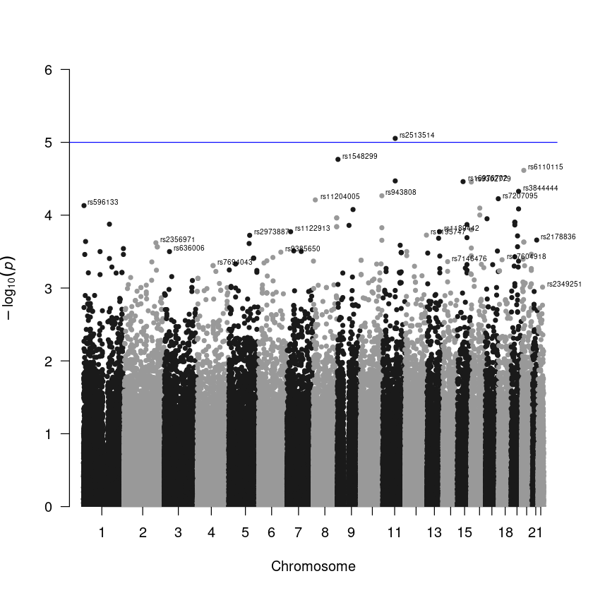
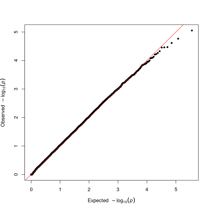
Step 4. Q-Q plot. The QQ plot serves as a crucial tool for identifying issues in a GWAS. To use it, input the vector of p-values from your association result into the qq() function.
qq(result$P)
There are more efficient ways to conduct association tests than using R. For instance, one can use well-developed software like PLINK. For more information, check this website. https://www.cog-genomics.org/plink/1.9/assoc
Step 1. Run association study by PLINK in the terminal.
#> plink --bfile human_all -assoc --out human_allStep 2. Read association test results (*.assoc) table by read.table() function.
library(data.table)
assoc = fread('../data/human/human_all.assoc')
head(assoc)| CHR | SNP | BP | A1 | F_A | F_U | A2 | CHISQ | P | OR |
|---|---|---|---|---|---|---|---|---|---|
| <int> | <chr> | <int> | <chr> | <dbl> | <dbl> | <chr> | <dbl> | <dbl> | <dbl> |
| 1 | rs3094315 | 792429 | G | 0.14890 | 0.08537 | A | 1.6840 | 0.1944 | 1.8750 |
| 1 | rs4040617 | 819185 | G | 0.13540 | 0.08537 | A | 1.1110 | 0.2919 | 1.6780 |
| 1 | rs4075116 | 1043552 | C | 0.04167 | 0.07317 | T | 0.8278 | 0.3629 | 0.5507 |
| 1 | rs9442385 | 1137258 | T | 0.37230 | 0.42680 | G | 0.5428 | 0.4613 | 0.7966 |
| 1 | rs11260562 | 1205233 | A | 0.02174 | 0.03659 | G | 0.3424 | 0.5585 | 0.5852 |
| 1 | rs6685064 | 1251215 | C | 0.38540 | 0.43900 | T | 0.5253 | 0.4686 | 0.8013 |
Step 3. Manhattan plot. The result table generated from PLINK is the exact format for the plotting function.
library(qqman)
manhattan(assoc)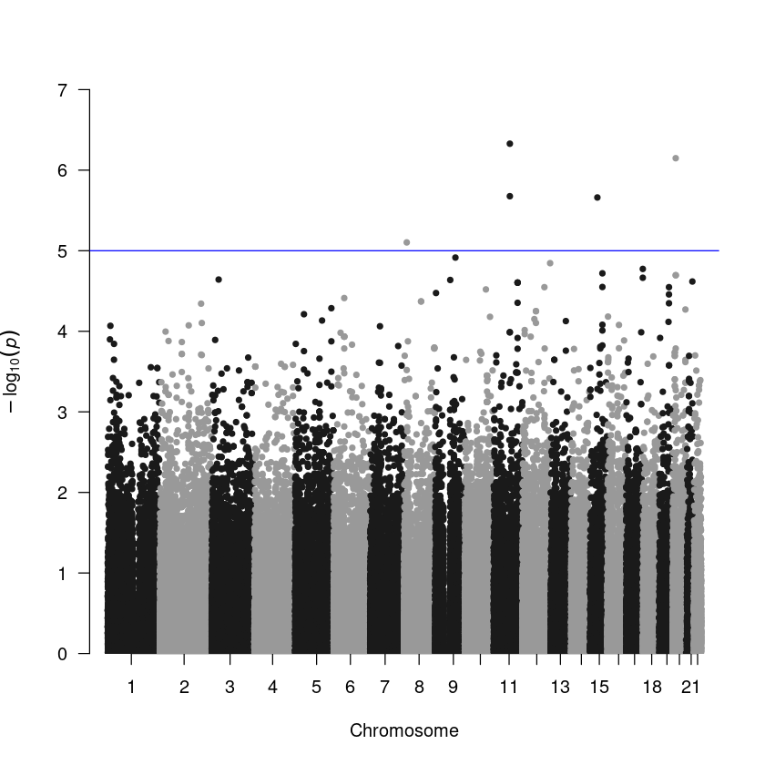
Step 4. Q-Q plot
qq(assoc$P)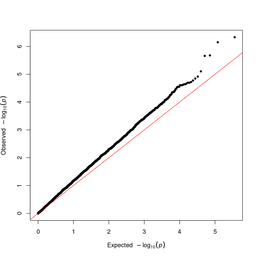
chisq.test()) and Yate’s correction for continuity (https://en.wikipedia.org/wiki/Yates%27s_correction_for_continuity).You can choose from different R packages for fitting GWAS linear mixed model. Some of these packages are GWAStools, rrBLUP, and sommer. Among these choices, my personal preference is the sommer package.
We will use a rice dataset from Cornell University in 2011 (https://www.nature.com/articles/ncomms1467). Raw data can be found on the rice diversity website (http://www.ricediversity.org/data/sets/44kgwas/).
library(sommer)Loading required package: Matrix
Loading required package: MASS
Loading required package: lattice
Attaching package: ‘lattice’
The following object is masked from ‘package:qqman’:
qq
Loading required package: crayon
Attaching package: ‘sommer’
The following object is masked from ‘package:qqman’:
manhattan
Read PLINK binary format files (rice.bed, rice.bim, rice.fam). This dataset contains various trait measurements. You can select one from the file rice_phenotype.txt and incorporate phenotype information into the fam data frame.
Read binary files by the genio() function.
data = read_plink('../data/rice44k/rice')Reading: ../data/rice44k/rice.bim
Reading: ../data/rice44k/rice.fam
Reading: ../data/rice44k/rice.bed
Read the phenotype table (I will choose plant height in the answer version)
peno = fread('../data/rice44k/rice_phenotype.txt')
peno = peno[, c(1, 13)]
colnames(peno) = c('id', 'pheno')
Merge data$fam and peno. The NSFTVID in the phenotype table is its individual ID.
data$fam$pheno = peno$pheno
peno = data$fam
Start preparing input data for the GWAS() function in the sommer() package.
geno = t(data$X) - 1
geno[is.na(geno)] = 0
peno$id = factor(peno$id)
Now we need to generate an additive relationship matrix using A.mat() function.
A = A.mat(geno)Then, we can fit the linear mixed model by the function GWAS()
fit = GWAS(fixed = pheno~1, random = ~vsr(id, Gu = A), data = peno, gTerm = "u:id", M = geno)Performing GWAS evaluationCreate a data frame for plotting the function. You should have CHR, SNP, BP, and P in four columns. The p-value could be calculated by 10^(-as.numeric(fit$scores))).
asso = data.frame(
    CHR = as.numeric(data$bim$chr),
    SNP = data$bim$id,
    BP = data$bim$pos,
    P = 10^(-as.numeric(fit$scores))
)
asso = asso[asso$P > 0, ]To create a Manhattan plot, please keep in mind that if the p-value is 0, its log value becomes infinity, which cannot be plotted. Therefore, kindly remove the data point before proceeding with the plot.
library(qqman)
qqman::manhattan(asso)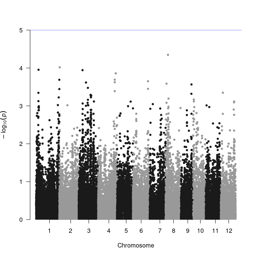
qqman::qq(result$P)